
Springs distribution
SSI has compiled available springs location data from many sources, and imported them into an ArcSDE geodatabase. We documented the information source for each spring, developed metadata according to best practice standards. We published the distribution data as a web mapping service (WMS), shown below, that is available by clicking here.
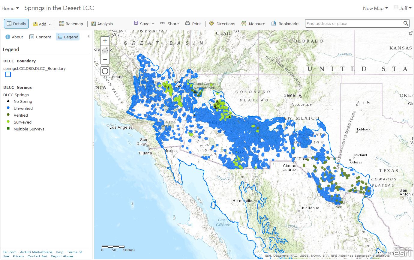
Interactive online map of publicly-available springs data within the Desert LCC. All data have been imported into the SpringsOnline database at http://springsdata.org/.
ANalysis of the DESERT lCc
Spatial datasets displayed in the maps below can be downloaded in a file geodatabase by clicking here.
anticipated Temperature change
Climate change has the potential to dramatically alter conditions in the Desert LCC Region. Increased temperatures and changes in precipitation patterns will likely cause shifts in species ranges, fractured species communities and extinctions of species that are unable to adapt or migrate.
In this map, HUCS are symbolized according to the median expected temperature change modeled for the years 2046-2065 under the A2 SRES Emissions Scenario, as determined by 16 Global Circulation Models used in the 2007 IPCC Fourth Assessment Report. Change is calculated from a baseline 1961-1990 mean of the 20th century simulation, 20C3M. HUC Temperature Change values are calculated as the weighted sum of intersecting climate model cells, where each model value is weighted according to the proportion of the cell lying within the HUC.
Click on a HUC polygon to see additional attributes including the Interquartile Range of model values, Seasonal expected values for April - September and October - March, and all temperature change statistics calculated from 17 GCMs under the B2 SRES Emissions scenario. Click Here to open the interactive map. ArcGIS users may Click Here to load data directly into ArcMap.
Variation in Temperature Models
The most defensible approach to estimate future conditions is to look at projections from multiple models, under multiple scenarios. We can then predict conditions for each scenario based on the model mean or median, and as a bonus we get an estimate of model agreement from the range, standard deviation and/or inter-quartile range of model predictions. Estimating conditions for each emissions scenario lets us compare the best-case prediction with the worst-case, and gives some sense of what we can hope for given our strategy for dealing with greenhouse gas emissions.
In this map, HUCS are symbolized according to the interquartile range of temperature change values predicted by 16 Global Circulation Models used in the 2007 IPCC Fourth Assessment Report. All models show conditions expected in the years 2046-2065 under the A2 SRES Emissions scenario. Change is calculated from a baseline 1961-1990 mean of the 20th century simulation, 20C3M. HUC Temperature Change values are calculated as the weighted sum of intersecting climate model cells, where each model value is weighted according to the proportion of the cell lying within the HUC.
Click on HUC polygons to see additional attributes including the median model value, Seasonal expected values for April - September and October - March, and all temperature change statistics calculated from 17 GCMs under the B2 SRES Emissions scenario. Click Here to open the interactive map at ArcGIS Online. ArcGIS users may Click Here to load data directly into ArcMap.
anticipated precipitation change
Climate change has the potential to dramatically alter conditions in the Desert LCC Region. Increased temperatures and changes in precipitation patterns will likely cause shifts in species ranges, fractured species communities and extinctions of species that are unable to adapt or migrate.
In this map, HUCS are symbolized according to the median expected change in precipitation modeled for the years 2046-2065 under the A2 SRES Scenario, as determined by 15 Global Circulation Models used in the 2007 IPCC Fourth Assessment Report. Change is calculated from a baseline 1961-1990 mean of the 20th century simulation, 20C3M. HUC Precipitation Change values are calculated as the weighted sum of intersecting climate model cells, where each model value is weighted according to the proportion of the cell lying within the HUC.
Click on a HUC polygon to see additional attributes including the Interquartile Range of model values, Seasonal expected values for April - September and October - March, and all precipitation change statistics calculated from 17 GCMS under the B2 SRES Emissions scenario. Click Here to open interactive map at ArcGIS Online. ArcGIS users may Click Here to load data directly into ArcMap.
variation in precipitation change models
The most defensible approach to estimate future conditions is to look at projections from multiple models, under multiple scenarios. We can then predict conditions for each scenario based on the model mean or median, and as a bonus we get an estimate of model agreement from the range, standard deviation and/or inter-quartile range of model predictions. Estimating conditions for each emissions scenario lets us compare the best-case prediction with the worst-case, and gives some sense of what we can hope for given our strategy for dealing with greenhouse gas emissions
In this map, HUCS are symbolized according to the interquartile range of precipitation change values predicted by 15 Global Circulation Models used in the 2007 IPCC Fourth Assessment Report. All models show conditions expected in the years 2046-2065 under the A2 SRES Emissions scenario. Change is calculated from a baseline 1961-1990 mean of the 20th century simulation, 20C3M. HUC Precipitation Change values are calculated as the weighted sum of intersecting climate model cells, where each model value is weighted according to the proportion of the cell lying within the HUC.
Click on HUC polygons to see additional attributes including the median model value, Seasonal expected values for April - September and October - March, and all precipitation change statistics calculated from 17 GCMS under the B2 SRES Emissions scenario. Click Here to view interactive map at ArcGIS Online. ArcGIS users may Click Here to load data directly into ArcMap.
species of concern
Here we show the number of species per HUC that are both sensitive and springs- or freshwater-dependent.
We examined all species found in the Springs Stewardship Institute Online Springs Database, and NatureServe's Map Viewer Dataset. We considered a species to be Springs- or Freshwater-Dependent if it met either of these two criteria:
- It had a Springs Stewardship Institute Springs Habitat Use value (if a plant) or Spring Life History value (if an invertebrate or vertebrate) of 4, 5 or 6 (meaning the species must have springs or springs-associated habitats to survive), or
- It had some evidence of freshwater-dependency in the NatureServe data attributes (specifically if it had non-null values for Lacustrine, Palustrine or Riverine, or if Subterranian (spp) value had "aquatic" in the name, or if the Special_Hab_Factor value had "benthic" in the name.
We considered a species to be sensitive if it met either of these two criteria:
- Again, if it had a Springs Habitat Use or Spring Life History value of 4, 5 or 6, or
- NatureServe ranked it as either "Imperiled" or "Vulnerable" according to NatureServe's Global Ranking system (Classes G1 - G3, T1 - T3; see NatureServe Global Ranks).
HUCS are symbolized according to the number of sensitive springs-dependent species known to exist in the HUC. Click on a HUC polygon to see a list of each species found in the HUC, along with additional attributes for each species. Click Here to view interactive map on ArcGIS Online. ArcGIS users may Click Here to load data directly into ArcMap.
species of concern, as a proportion of all species
Here we show the number of species per HUC that are both sensitive and springs- or freshwater-dependent, divided by the total number of species found in the HUC.
We examined all species found in the Springs Stewardship Institute Online Springs Database, and NatureServe's Map Viewer Dataset. We considered a species to be Springs- or Freshwater-Dependent if it met either of these two criteria:
- It had a Springs Stewardship Institute Springs Habitat Use value (if a plant) or Spring Life History value (if an invertebrate or vertebrate) of 4, 5 or 6 (meaning the species must have springs or springs-associated habitats to survive), or
- It had some evidence of freshwater-dependency in the NatureServe data attributes (specifically if it had non-null values for Lacustrine, Palustrine or Riverine, or if Subterranian (spp) value had "aquatic" in the name, or if the Special_Hab_Factor value had "benthic" in the name.
We considered a species to be sensitive if it met either of these two criteria:
- Again, if it had a Springs Habitat Use or Spring Life History value of 4, 5 or 6, or
- NatureServe ranked it as either "Imperiled" or "Vulnerable" according to NatureServe's Global Ranking system (Classes G1 - G3, T1 - T3; see NatureServe Global Ranks).
HUCS are symbolized according to the proportion of sensitive springs-dependent species known to exist in the HUC, divided by the total number of species found in the HUC. Click on a HUC polygon to see a list of each sensitive and freshwater-dependent species found in the HUC, along with additional attributes for each species. Click Here to view the interactive online map. ArcGIS users may Click Here to load data directly into ArcMap.
population density 1990
HUCS are symbolized according to the population density in 1990, as determined by US Census Block data (available here and here). HUC populations are calculated as the weighted sum of intersecting census block populations, where each block population is weighted according to the proportion of the block lying within the HUC. Populations are then divided by the area of the HUC (in Square Kilometers) to get the density.
Click on a HUC polygon to see additional attributes including the populations at 1990, 2000 and 2010, the population densities in 2000 and 2010, and the rates of population change for the time periods [1990 - 2000], [2000 - 2010] and [1990 - 2010]. Click Here to view the online interactive map. ArcGIS users may Click Here to load data directly into ArcMap.
population density 2000
HUCS are symbolized according to the population density in 2000, as determined by US Census Block data (available here and here). HUC populations are calculated as the weighted sum of intersecting census block populations, where each block population is weighted according to the proportion of the block lying within the HUC. Populations are then divided by the area of the HUC (in Square Kilometers) to get the density.
Click on a HUC polygon to see additional attributes including the populations at 1990, 2000 and 2010, the population densities in 1990 and 2010, and the rates of population change for the time periods [1990 - 2000], [2000 - 2010] and [1990 - 2010]. Click Here to view the online interactive map. ArcGIS users may Click Here to load data directly into ArcMap.
population density 2010
HUCS are symbolized according to the population density in 2010, as determined by US Census Block data available here, here and here). HUC populations are calculated as the weighted sum of intersecting census block populations, where each block population is weighted according to the proportion of the block lying within the HUC. Populations are then divided by the area of the HUC (in Square Kilometers) to get the density.
Click on a HUC polygon to see additional attributes including the populations at 1990, 2000 and 2010, the population densities in 1990 and 2000, and the rates of population change for the time periods [1990 - 2000], [2000 - 2010] and [1990 - 2010]. Click Here to view the online interactive map. ArcGIS users may Click Here to load data directly into ArcMap.
POPULATION RATE OF CHANGE: 1990 - 2010
HUCS are symbolized according to the population population rate of change between 1990 and 2010, as determined by US Census Block data for 1990 (available here and here) and 2010 (available here, here and here).
HUC populations are calculated as the weighted sum of intersecting census block populations, where each block population is weighted according to the proportion of the block lying within the HUC. Populations are then divided by the area of the HUC (in Square Kilometers) to get the density. Population Rate of Change is defined as the ratio of the 2010 population divided by the 1990 population. A value of 100% means the population has remained unchanged.
Click on a HUC polygon to see additional attributes including the populations at 1990, 2000 and 2010, the population densities in 1990, 2000 and 2010, and the rates of population change for the time periods [1990 - 2000] and [2000 - 2010]. Click Here to view the online interactive map. ArcGIS users may Click Here to load data directly into ArcMap.